Exploratory analysis using group

Data sets can frequently be partitioned into meaningful groups based on the variables they contain. Making this grouping explicit allows the computation of numeric summaries within groups, which in turn facilitates quantitative comparisons.

This is the second module in the Visualization and EDA topic; the relevant slack channel is here.

Some slides

Exploratory Analysis from Jeff Goldsmith.

Example

We’ll continue in the same project that we used for visualization, and use essentially the same dataset – the only exception is the addition of month variable, created using lubridate::floor_date().

library(rnoaa)

weather = 
  meteo_pull_monitors(c("USW00094728", "USC00519397", "USS0023B17S"),
                      var = c("PRCP", "TMIN", "TMAX"), 
                      date_min = "2016-01-01",
                      date_max = "2016-12-31") %>%
  mutate(
    name = recode(id, USW00094728 = "CentralPark_NY", 
                      USC00519397 = "Waikiki_HA",
                      USS0023B17S = "Waterhole_WA"),
    tmin = tmin / 10,
    tmax = tmax / 10,
    month = lubridate::floor_date(date, unit = "month")) %>%
  select(name, id, date, month, everything())
weather
## # A tibble: 1,098 x 7
##              name          id       date      month  prcp  tmax  tmin
##             <chr>       <chr>     <date>     <date> <dbl> <dbl> <dbl>
##  1 CentralPark_NY USW00094728 2016-01-01 2016-01-01     0   5.6   1.1
##  2 CentralPark_NY USW00094728 2016-01-02 2016-01-01     0   4.4   0.0
##  3 CentralPark_NY USW00094728 2016-01-03 2016-01-01     0   7.2   1.7
##  4 CentralPark_NY USW00094728 2016-01-04 2016-01-01     0   2.2  -9.9
##  5 CentralPark_NY USW00094728 2016-01-05 2016-01-01     0  -1.6 -11.6
##  6 CentralPark_NY USW00094728 2016-01-06 2016-01-01     0   5.0  -3.8
##  7 CentralPark_NY USW00094728 2016-01-07 2016-01-01     0   7.8  -0.5
##  8 CentralPark_NY USW00094728 2016-01-08 2016-01-01     0   7.8  -0.5
##  9 CentralPark_NY USW00094728 2016-01-09 2016-01-01     0   8.3   4.4
## 10 CentralPark_NY USW00094728 2016-01-10 2016-01-01   457  15.0   4.4
## # ... with 1,088 more rows

`group_by`

Datasets are often comprised of groups defined by one or more (categorical) variable; group_by() makes these groupings explicit so that they can be included in subsequent operations. For example, we might group weather by name and month:

weather %>%
  group_by(name, month)
## # A tibble: 1,098 x 7
## # Groups:   name, month [36]
##   name           id          date       month       prcp  tmax  tmin
##   <chr>          <chr>       <date>     <date>     <dbl> <dbl> <dbl>
## 1 CentralPark_NY USW00094728 2016-01-01 2016-01-01     0   5.6   1.1
## 2 CentralPark_NY USW00094728 2016-01-02 2016-01-01     0   4.4   0  
## 3 CentralPark_NY USW00094728 2016-01-03 2016-01-01     0   7.2   1.7
## 4 CentralPark_NY USW00094728 2016-01-04 2016-01-01     0   2.2  -9.9
## 5 CentralPark_NY USW00094728 2016-01-05 2016-01-01     0  -1.6 -11.6
## 6 CentralPark_NY USW00094728 2016-01-06 2016-01-01     0   5    -3.8
## # ... with 1,092 more rows

Several important functions respect grouping structures. You will frequently use summarize to create one-number summaries within each group, or use mutate to define variables within groups. The rest of this example shows these functions in action.

Because these (and other) functions will use grouping information if it exists, it is sometimes necessary to remove groups using ungroup().

Counting things

As an intro to summarize, let’s count the number of observations in each month in the complete weather dataset.

weather %>%
  group_by(month) %>%
  summarize(n = n())
## # A tibble: 12 x 2
##    month          n
##    <date>     <int>
##  1 2016-01-01    93
##  2 2016-02-01    87
##  3 2016-03-01    93
##  4 2016-04-01    90
##  5 2016-05-01    93
##  6 2016-06-01    90
##  7 2016-07-01    93
##  8 2016-08-01    93
##  9 2016-09-01    90
## 10 2016-10-01    93
## 11 2016-11-01    90
## 12 2016-12-01    93

The result is a dataframe that includes the grouping variable and the desired summary.

In this case, you could use count() in place of group_by() and summarize() if you remember that this function exists.

weather %>%
  count(month)
## # A tibble: 12 x 2
##    month          n
##    <date>     <int>
##  1 2016-01-01    93
##  2 2016-02-01    87
##  3 2016-03-01    93
##  4 2016-04-01    90
##  5 2016-05-01    93
##  6 2016-06-01    90
##  7 2016-07-01    93
##  8 2016-08-01    93
##  9 2016-09-01    90
## 10 2016-10-01    93
## 11 2016-11-01    90
## 12 2016-12-01    93

You can use summarize() to compute multiple summaries within each group. As an example, we count the number of observations in each month and the number of distinct values of date in each month.

weather %>%
  group_by(month) %>%
  summarize(n_obs = n(),
            n_days = n_distinct(date))
## # A tibble: 12 x 3
##    month      n_obs n_days
##    <date>     <int>  <int>
##  1 2016-01-01    93     31
##  2 2016-02-01    87     29
##  3 2016-03-01    93     31
##  4 2016-04-01    90     30
##  5 2016-05-01    93     31
##  6 2016-06-01    90     30
##  7 2016-07-01    93     31
##  8 2016-08-01    93     31
##  9 2016-09-01    90     30
## 10 2016-10-01    93     31
## 11 2016-11-01    90     30
## 12 2016-12-01    93     31

General summaries

Standard statistical summaries are regularly computed in summarize() using functions like mean(), median(), var(), sd(), mad(), IQR(), min(), and max(). To use these, you indicate the variable to which they apply and include any additional arguments as necessary.

weather %>%
  group_by(month) %>%
  summarize(mean_tmax = mean(tmax),
            mean_prec = mean(prcp, na.rm = TRUE),
            median_tmax = median(tmax),
            sd_tmax = sd(tmax))
## # A tibble: 12 x 5
##    month      mean_tmax mean_prec median_tmax sd_tmax
##    <date>         <dbl>     <dbl>       <dbl>   <dbl>
##  1 2016-01-01      11.6      50.4         5     12.4 
##  2 2016-02-01      13.2      38.9         8.8   12.1 
##  3 2016-03-01      15.4      42.9        13.3   11.2 
##  4 2016-04-01      18.6      11.5        18.3    9.63
##  5 2016-05-01      20.9      15.8        21.1    8.92
##  6 2016-06-01      23.4      16.6        28.3    8.61
##  7 2016-07-01      25.1      39.5        29.4    8.14
##  8 2016-08-01      26.0      11.5        30      7.02
##  9 2016-09-01      22.7      19.1        26.7    8.74
## 10 2016-10-01      18.1      51.5        18.3   10.5 
## 11 2016-11-01      15.4      72.1        14.7   10.8 
## 12 2016-12-01      10.4      36.5         7.8   13.1

You can group by more than one variable.

weather %>%
  group_by(name, month) %>%
  summarize(mean_tmax = mean(tmax),
            median_tmax = median(tmax))
## # A tibble: 36 x 4
## # Groups:   name [?]
##   name           month      mean_tmax median_tmax
##   <chr>          <date>         <dbl>       <dbl>
## 1 CentralPark_NY 2016-01-01      4.89         5  
## 2 CentralPark_NY 2016-02-01      7.14         5  
## 3 CentralPark_NY 2016-03-01     14.1         13.3
## 4 CentralPark_NY 2016-04-01     16.8         16.7
## 5 CentralPark_NY 2016-05-01     21.5         21.1
## 6 CentralPark_NY 2016-06-01     27.2         28.3
## # ... with 30 more rows

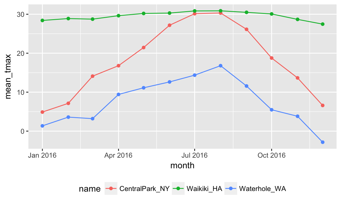
The fact that summarize() produces a dataframe is important (and consistent with other functions in the tidyverse). You can incorporate grouping and summarizing within broader analysis pipelines. For example, we can take create a plot based on the monthly summary:

weather %>%
  group_by(name, month) %>%
  summarize(mean_tmax = mean(tmax)) %>%
  ggplot(aes(x = month, y = mean_tmax, color = name)) + 
    geom_point() + geom_line() + 
    theme(legend.position = "bottom")

Grouped `mutate`

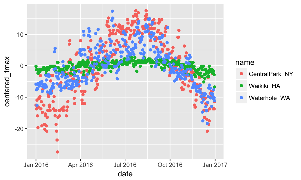
Summarizing collapses groups into single data points. In contrast, using mutate() in conjuntion with group_by() will retain all original data points and add new variables computed within groups.

Suppose you want to compare the daily max temperature to the annual average max temperature for each station separately, and to plot the result. You could do so using:

weather %>%
  group_by(name) %>%
  mutate(centered_tmax = tmax - mean(tmax)) %>% 
  ggplot(aes(x = date, y = centered_tmax, color = name)) + 
    geom_point()

Window functions

The previous example used mean() to compute the mean within each group, which was then subtracted from the observed max tempurature. mean() takes n inputs and produces a single output.

Window functions, in contrast, take n inputs and return n outputs, and the outputs depend on all the inputs. There are several categories of window functions; you’re most likely to need ranking functions and offsets, which we illustrate below.

First, we can find the max temperature ranking within month.

weather %>%
  group_by(name, month) %>%
  mutate(temp_ranking = min_rank(tmax))
## # A tibble: 1,098 x 8
## # Groups:   name, month [36]
##   name       id       date       month       prcp  tmax  tmin temp_ranking
##   <chr>      <chr>    <date>     <date>     <dbl> <dbl> <dbl>        <int>
## 1 CentralPa… USW0009… 2016-01-01 2016-01-01     0   5.6   1.1           18
## 2 CentralPa… USW0009… 2016-01-02 2016-01-01     0   4.4   0             14
## 3 CentralPa… USW0009… 2016-01-03 2016-01-01     0   7.2   1.7           22
## 4 CentralPa… USW0009… 2016-01-04 2016-01-01     0   2.2  -9.9            8
## 5 CentralPa… USW0009… 2016-01-05 2016-01-01     0  -1.6 -11.6            3
## 6 CentralPa… USW0009… 2016-01-06 2016-01-01     0   5    -3.8           16
## # ... with 1,092 more rows

This sort of ranking is useful when filtering data based on rank. We could, for example, keep only the day with the lowest max temperature within each month:

weather %>%
  group_by(name, month) %>%
  filter(min_rank(tmax) < 2)
## # A tibble: 47 x 7
## # Groups:   name, month [36]
##   name           id          date       month       prcp  tmax  tmin
##   <chr>          <chr>       <date>     <date>     <dbl> <dbl> <dbl>
## 1 CentralPark_NY USW00094728 2016-01-23 2016-01-01   587  -2.7  -4.3
## 2 CentralPark_NY USW00094728 2016-02-14 2016-02-01     0  -9.3 -18.2
## 3 CentralPark_NY USW00094728 2016-03-03 2016-03-01     0   2.2  -3.2
## 4 CentralPark_NY USW00094728 2016-04-05 2016-04-01     0   6.1  -3.2
## 5 CentralPark_NY USW00094728 2016-04-09 2016-04-01    28   6.1   2.2
## 6 CentralPark_NY USW00094728 2016-05-01 2016-05-01    41  10.6   7.2
## # ... with 41 more rows

We could also keep the three days with the highest max temperature:

weather %>%
  group_by(name, month) %>%
  filter(min_rank(desc(tmax)) < 4)
## # A tibble: 151 x 7
## # Groups:   name, month [36]
##   name           id          date       month       prcp  tmax  tmin
##   <chr>          <chr>       <date>     <date>     <dbl> <dbl> <dbl>
## 1 CentralPark_NY USW00094728 2016-01-10 2016-01-01   457  15     4.4
## 2 CentralPark_NY USW00094728 2016-01-16 2016-01-01    61  11.1   5.6
## 3 CentralPark_NY USW00094728 2016-01-31 2016-01-01     0  13.3   2.2
## 4 CentralPark_NY USW00094728 2016-02-20 2016-02-01     0  16.1   3.9
## 5 CentralPark_NY USW00094728 2016-02-25 2016-02-01     5  16.1   2.8
## 6 CentralPark_NY USW00094728 2016-02-29 2016-02-01    13  16.1   8.3
## # ... with 145 more rows

In both of these, we’ve skipped a mutate() statement that would create a ranking variable, and gone straight to filtering based on the result.

Offsets, especially lags, are used to compare an observation to it’s previous value. This is useful, for example, to find the day-by-day change in max temperature within each station over the year:

weather %>%
  group_by(name) %>%
  mutate(temp_change = tmax - lag(tmax))
## # A tibble: 1,098 x 8
## # Groups:   name [3]
##   name           id    date       month       prcp  tmax  tmin temp_change
##   <chr>          <chr> <date>     <date>     <dbl> <dbl> <dbl>       <dbl>
## 1 CentralPark_NY USW0… 2016-01-01 2016-01-01     0   5.6   1.1       NA   
## 2 CentralPark_NY USW0… 2016-01-02 2016-01-01     0   4.4   0         -1.20
## 3 CentralPark_NY USW0… 2016-01-03 2016-01-01     0   7.2   1.7        2.8 
## 4 CentralPark_NY USW0… 2016-01-04 2016-01-01     0   2.2  -9.9       -5   
## 5 CentralPark_NY USW0… 2016-01-05 2016-01-01     0  -1.6 -11.6       -3.8 
## 6 CentralPark_NY USW0… 2016-01-06 2016-01-01     0   5    -3.8        6.6 
## # ... with 1,092 more rows

This kind of variable might be used to quantify the day-by-day variability in max temperature, or to identify the largest one-day increase:

weather %>%
  group_by(name) %>%
  mutate(temp_change = tmax - lag(tmax)) %>%
  summarize(temp_change_sd = sd(temp_change, na.rm = TRUE),
            temp_change_max = max(temp_change, na.rm = TRUE))
## # A tibble: 3 x 3
##   name           temp_change_sd temp_change_max
##   <chr>                   <dbl>           <dbl>
## 1 CentralPark_NY           4.28            12.2
## 2 Waikiki_HA               1.15             5  
## 3 Waterhole_WA             2.82             9

Limitations

summarize() can only be used with functions that return a single-number summary. This creates a ceiling, even if it is very high. Later we’ll see how to aggregate data in a more general way, and how to perform complex operations on the resulting sub-datasets.

Other materials

The preceding is based heavily on Jenny Bryan’s group_by material
R for Data Science has sub-chapters on grouped summaries and exploratory data analysis
A more in-depth overview of window functions is here

The code that I produced working examples in lecture is here.

Exploratory analysis using group_by