Strings and factors

library(tidyverse)
library(janitor)
library(haven)
library(rvest)

library(stringr)
library(forcats)

theme_set(theme_bw())
theme_update(legend.position = "bottom")

PULSE data

We’ll start by revisiting a dataset we’ve seen a few times now. In tidy data we spent some time tidying the PULSE dataset; as part of that we used tools available to us at the time, but now we have some better tools.

The code below updates the data processing pipeline for the PULSE data using strignr and forcats. The result is the same, and the differences are pretty small, but this is a bit cleaner.

pulse_data = read_sas("./data/public_pulse_data.sas7bdat") %>%
  clean_names() %>%
  gather(key = visit, value = bdi, bdi_score_bl:bdi_score_12m) %>%
  mutate(visit = str_replace(visit, "bdiscore_", ""),
         visit = str_replace(visit, "bl", "00m"),
         visit = fct_relevel(visit, str_c(c("00", "01", "06", "12"), "m"))) %>%
  arrange(id, visit)
## Warning: attributes are not identical across measure variables;
## they will be dropped
## Warning: Unknown levels in `f`: 00m, 01m, 06m, 12m

print(pulse_data, n = 12)
## # A tibble: 4,348 x 5
##       id   age sex   visit           bdi
##    <dbl> <dbl> <chr> <fct>         <dbl>
##  1 10003  48.0 male  bdi_score_00m     7
##  2 10003  48.0 male  bdi_score_01m     1
##  3 10003  48.0 male  bdi_score_06m     2
##  4 10003  48.0 male  bdi_score_12m     0
##  5 10015  72.5 male  bdi_score_00m     6
##  6 10015  72.5 male  bdi_score_01m    NA
##  7 10015  72.5 male  bdi_score_06m    NA
##  8 10015  72.5 male  bdi_score_12m    NA
##  9 10022  58.5 male  bdi_score_00m    14
## 10 10022  58.5 male  bdi_score_01m     3
## 11 10022  58.5 male  bdi_score_06m     8
## 12 10022  58.5 male  bdi_score_12m    NA
## # ... with 4,336 more rows

NSDUH

Next we’ll revisit the table scraped from the National Survey on Drug Use and Health data on this page. In reading data from the web, we loaded this data using the code below, but noted it wasn’t tidy.

url = "http://samhda.s3-us-gov-west-1.amazonaws.com/s3fs-public/field-uploads/2k15StateFiles/NSDUHsaeShortTermCHG2015.htm"
drug_use_xml = read_html(url)

table_marj = (drug_use_xml %>% html_nodes(css = "table"))[[1]] %>%
  html_table() %>%
  .[-1,] %>%
  as_tibble()

There are a few steps we need to implement to tidy these data. For now I’m not interested in the p-values (I’d rather just see the data); we also have age groups and year ranges in column titles, both of which are, in fact, variables. Lastly, the table includes letters as superscripts next to table entries; if we only want the percents we’ll need to strip these out.

data_marj = 
  table_marj %>%
  select(-contains("P Value")) %>%
  gather(key = key, value = percent, -State) %>%
  separate(key, into = c("age", "year"), sep = "\\(") %>%
  mutate(year = str_sub(year, 1, -2),
         percent = str_replace(percent, "[a-z]", ""),
         percent = as.numeric(percent)) %>%
  filter(!(State %in% c("Total U.S.", "Northeast", "Midwest", "South", "West")))

We used stringr and regular expressions a couple of times above:

• in separate, we split age and year at the open parentheses using "\\("
• to remove character superscripts, we replaced any character using "[a-z]"

Let’s quickly visualize these data for the 12-17 age group; to make the plot readable, we’ll treat State as a factor are reorder according to percent.

data_marj %>%
  filter(age == "12-17") %>% 
  mutate(State = fct_reorder(State, percent)) %>% 
  ggplot(aes(x = State, y = percent, color = year)) + 
    geom_point() + 
    theme(axis.text.x = element_text(angle = 90, hjust = 1))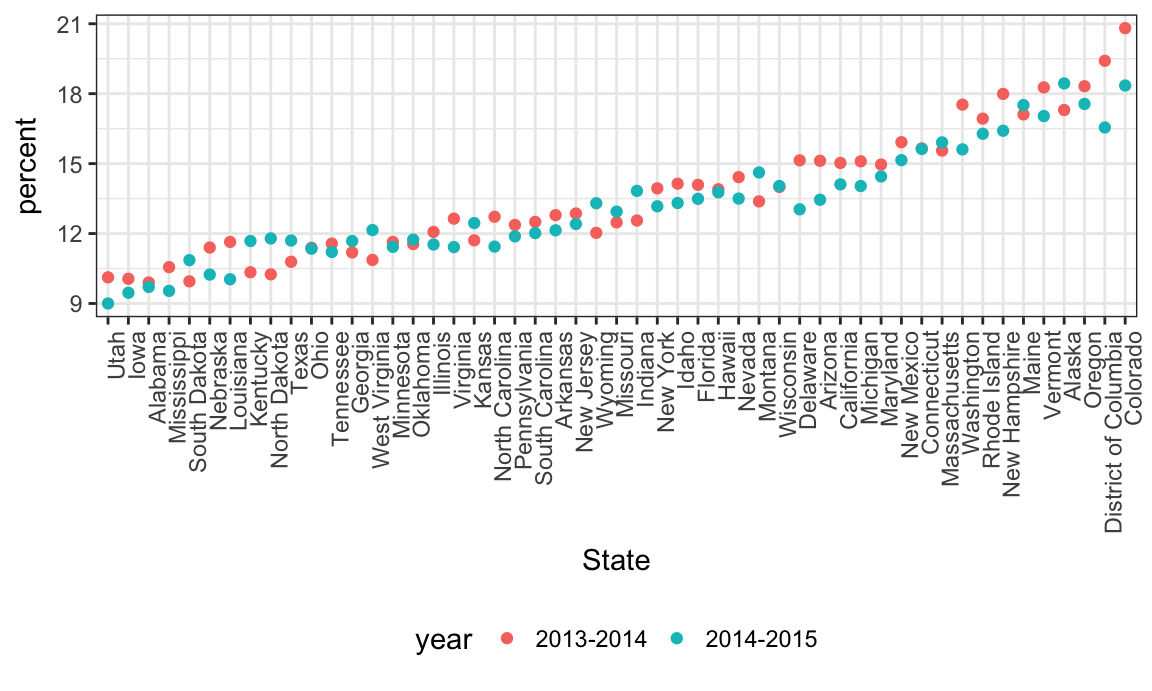

Toothbrush reviews

We were able to scrape toothbrush reviews for a single review page in reading data from the web. If we want to scrape more reviews, it’s necessary to construct the URLs for several review pages. This is possible based on an observation about the the structure of the URL for the first page of reviews – it ended with pageNumber=1 and, sure enough, changing this to pageNumber=2 will bring up the second page of reviews.

url_base = "https://www.amazon.com/Philips-Sonicare-rechargeable-toothbrush-HX6211/product-reviews/B00YAR7ZFM/ref=cm_cr_arp_d_viewopt_srt?ie=UTF8&reviewerType=all_reviews&sortBy=recent&pageNumber="

urls = str_c(url_base, 1:5)

read_html(urls[1]) %>% 
  html_nodes("#cm_cr-review_list .review-title") %>%
  html_text()
##  [1] "Five Stars"                                          
##  [2] "The BEST Toothbrush"                                 
##  [3] "Five Stars"                                          
##  [4] "It doesn't clean as good as the round spinning brush"
##  [5] "Five Stars"                                          
##  [6] "One Star"                                            
##  [7] "Ni-MH battery, NOT LITHIUM!"                         
##  [8] "I wasted my money"                                   
##  [9] "but still works fine. Great for the price"           
## [10] "Four Stars"

read_html(urls[2]) %>% 
  html_nodes("#cm_cr-review_list .review-title") %>%
  html_text()
##  [1] "Still working perfectly nearly two years later"           
##  [2] "Five Stars"                                               
##  [3] "Significant difference in clean teeth/gums"               
##  [4] "Five Stars"                                               
##  [5] "Five Stars"                                               
##  [6] "A good buy"                                               
##  [7] "Works great, love it"                                     
##  [8] "One Star"                                                 
##  [9] "... each of the members in my household and we love them."
## [10] "Bad battery"

It would get really tedious to try to scrape all (5000+) reviews by copying code over and over; before long we’ll learn about writing R functions to reuse code and make this much easier!

Biostat Methods I Example

The following dataset was used as an example in Biostat Methods on ANOVA. First we’ll recreate the dataset.

ins1 = c(1.53, 1.61, 3.75, 2.89, 3.26)
ins2 = c(3.15, 3.96, 3.59, 1.89, 1.45, 1.56)
ins3 = c(3.89, 3.68, 5.70, 5.62, 5.79, 5.33)
ins4 = c(8.18, 5.64, 7.36, 5.33, 8.82, 5.26, 7.10)
ins5 = c(5.86, 5.46, 5.69, 6.49, 7.81, 9.03, 7.49, 8.98)

bmi_data = data_frame(
    insulin = c(ins1, ins2, ins3, ins4, ins5),
    ind = c(rep(1, length(ins1)),
                    rep(2, length(ins2)),
                    rep(3, length(ins3)),
                    rep(4, length(ins4)),
                    rep(5, length(ins5)))
)

Next we’ll convert ind to a factor variable with informative levels, make a quick plot, and fit a linear model using ind as a predictor and insulin as the outcome.

bmi_data = bmi_data %>% 
  mutate(ind = factor(ind), 
         ind = fct_recode(ind,
                          "level_1" = "1",
                          "level_2" = "2",
                          "level_3" = "3",
                          "level_4" = "4",
                          "level_5" = "5")
         )

bmi_data %>% 
  ggplot(aes(x = ind, y = insulin)) + geom_boxplot()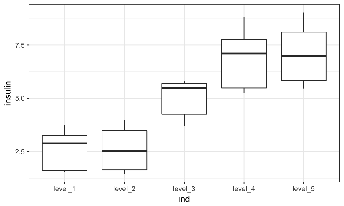

bmi_data %>% 
  lm(insulin ~ ind, data = .) %>% 
  broom::tidy() %>% 
  select(-std.error, -statistic) %>% 
  knitr::kable(digits = 3)

term	estimate	p.value
(Intercept)	2.608	0.000
indlevel_2	-0.008	0.992
indlevel_3	2.394	0.004
indlevel_4	4.205	0.000
indlevel_5	4.493	0.000

As it is, level_1 is used as the reference group in the regression model. That might make sense, and it might not – if the factor takes on different values you may want something else as the reference.

bmi_data = bmi_data %>% 
  mutate(ind = fct_recode(ind,
                          "very_low"  = "level_1",
                          "low"       = "level_2",
                          "neutral"   = "level_3",
                          "high"      = "level_4",
                          "very_high" = "level_5"),
         ind = fct_relevel(ind, "neutral"))

bmi_data %>% 
  lm(insulin ~ ind, data = .) %>% 
  broom::tidy() %>% 
  select(-std.error, -statistic) %>% 
  knitr::kable(digits = 3)

term	estimate	p.value
(Intercept)	5.002	0.000
indvery_low	-2.394	0.004
indlow	-2.402	0.002
indhigh	1.811	0.014
indvery_high	2.100	0.004

Shifting the reference category also changes our plot.

bmi_data %>% 
  ggplot(aes(x = ind, y = insulin)) + geom_boxplot()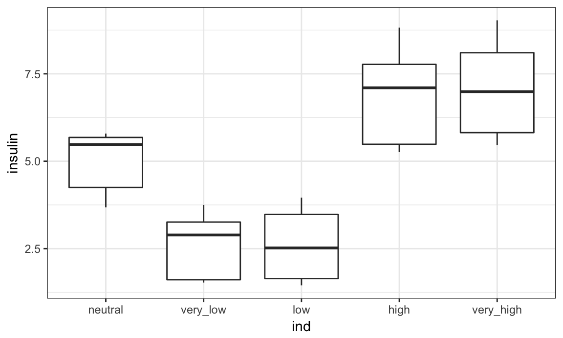

In the above example, neutral makes sense as a reference group but might not give the ordering you want for visualizations. That’s fine – you can use what you need when you need it!

Restaurant inspections

As a final example of strings and factors, we’ll take a look at the NYC Restuarant Inspections data. Although we won’t talk about this in detail now, it’s worth mentioning that these data were collected using the NYC Open Data API; code is available with the data description.

First we’ll import the data and take a look.

nyc_inspections = read_csv("./data/DOHMH_New_York_City_Restaurant_Inspection_Results.csv.gz", 
                           col_types = cols(building = col_character()),
                           na = c("NA", "N/A"))

nyc_inspections %>% 
  group_by(boro, grade) %>% 
  summarize(n = n()) %>% 
  spread(key = grade, value = n)
## # A tibble: 6 x 8
## # Groups:   boro [6]
##   boro              A     B     C `Not Yet Graded`     P     Z `<NA>`
##   <chr>         <int> <int> <int>            <int> <int> <int>  <int>
## 1 BRONX         13688  2801   701              200   163   351  16833
## 2 BROOKLYN      37449  6651  1684              702   416   977  51930
## 3 MANHATTAN     61608 10532  2689              765   508  1237  80615
## 4 Missing           4    NA    NA               NA    NA    NA     13
## 5 QUEENS        35952  6492  1593              604   331   913  45816
## 6 STATEN ISLAND  5215   933   207               85    47   149   6730

To simplify things, I’ll remove inspections with scores other than A, B, or C, and also remove the restaurants with missing boro information. I’ll also clean up boro names a bit.

nyc_inspections =
  nyc_inspections %>%
  filter(grade %in% c("A", "B", "C"), boro != "Missing") %>% 
  mutate(boro = str_to_title(boro))

Let’s focus only on pizza places for now, and re-examine grades by boro

nyc_inspections %>% 
  filter(str_detect(dba, "Pizza")) %>% 
  group_by(boro, grade) %>% 
  summarize(n = n()) %>% 
  spread(key = grade, value = n)
## # A tibble: 5 x 3
## # Groups:   boro [5]
##   boro              A     B
##   <chr>         <int> <int>
## 1 Bronx             9     3
## 2 Brooklyn          6    NA
## 3 Manhattan        26     8
## 4 Queens           17    NA
## 5 Staten Island     5    NA

That doesn’t look right – for sure there are more pizza places than that! The problem is that the match in str_detect is case-sensitive until we tell it not to be:

nyc_inspections %>% 
  filter(str_detect(dba, regex("pizza", ignore_case = TRUE))) %>% 
  group_by(boro, grade) %>% 
  summarize(n = n()) %>% 
  spread(key = grade, value = n)
## # A tibble: 5 x 4
## # Groups:   boro [5]
##   boro              A     B     C
##   <chr>         <int> <int> <int>
## 1 Bronx          1170   305    56
## 2 Brooklyn       1948   296    61
## 3 Manhattan      1983   420    76
## 4 Queens         1647   259    48
## 5 Staten Island   323   127    21

The table is okay but I’d like to visualize this.

nyc_inspections %>% 
  filter(str_detect(dba, regex("pizza", ignore_case = TRUE))) %>%
  ggplot(aes(x = boro, fill = grade)) + geom_bar()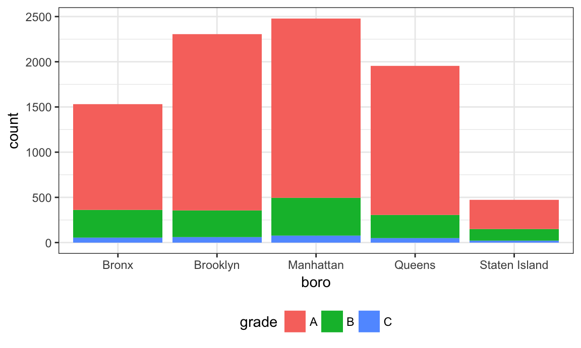

Might help to have things in a different order – maybe number of pizza places? Fortunately this can be done using fct_infreq.

nyc_inspections %>% 
  filter(str_detect(dba, regex("pizza", ignore_case = TRUE))) %>%
  mutate(boro = fct_infreq(boro)) %>%
  ggplot(aes(x = boro, fill = grade)) + geom_bar()

Suppose I want to rename a boro; I’ll try to do this using replace.

nyc_inspections %>% 
  filter(str_detect(dba, regex("pizza", ignore_case = TRUE))) %>%
  mutate(boro = fct_infreq(boro),
         boro = replace(boro, which(boro == "Brooklyn"), "Hipsterville")) %>%
  ggplot(aes(x = boro, fill = grade)) + geom_bar()
## Warning in `[<-.factor`(`*tmp*`, list, value = "Hipsterville"): invalid
## factor level, NA generated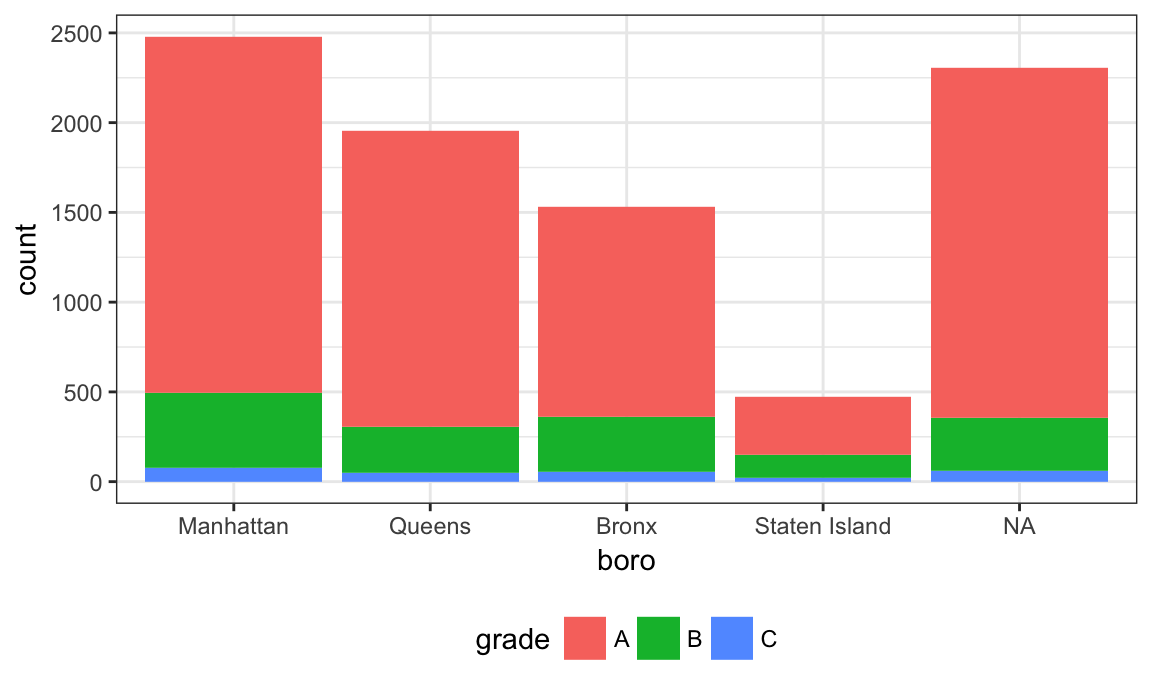

That didn’t work at all! Factors have very specific values, trying to use a value that is not an existing factor level won’t work. Fortunately there is a dedicated function for renaming factor levels:

nyc_inspections %>% 
  filter(str_detect(dba, regex("pizza", ignore_case = TRUE))) %>%
  mutate(boro = fct_infreq(boro),
         boro = fct_recode(boro, "Hipsterville" = "Brooklyn")) %>%
  ggplot(aes(x = boro, fill = grade)) + geom_bar()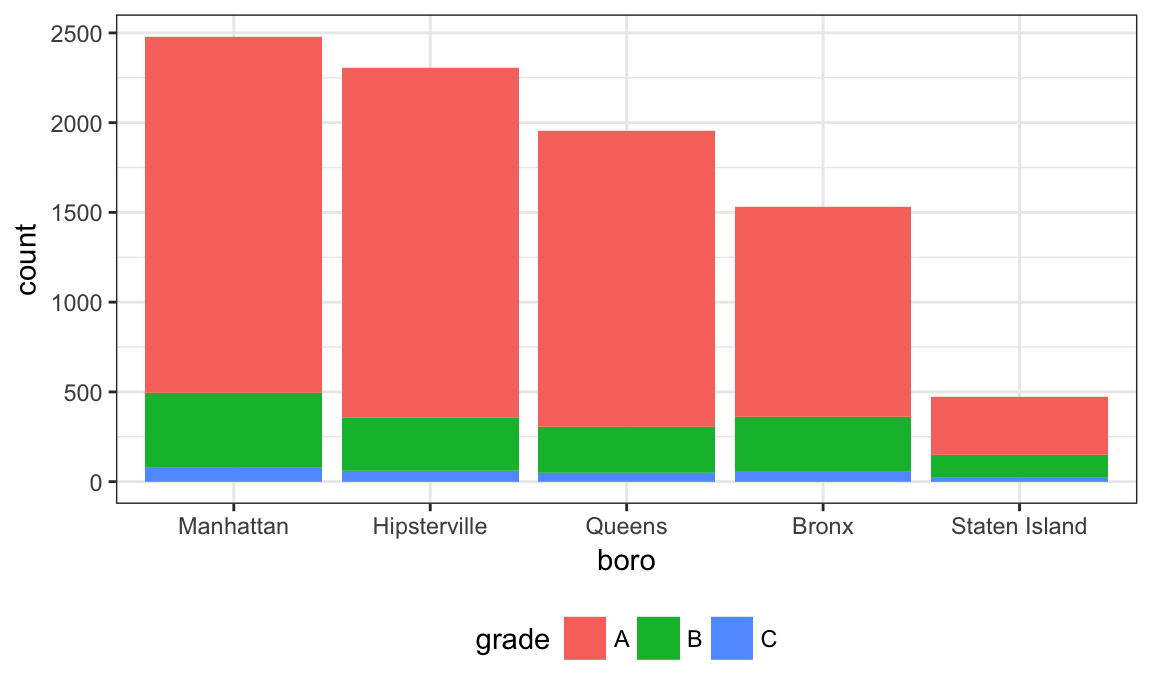

Success!