Notation for FDA

This page contains a combination of traditional lecture materials (slides) and code demonstrating the relevant methods. The short course will proceed by working through both. We will use several recent packages in our examples; see the About page for information about the package versions.

library(tidyverse)
library(refund.shiny)

theme_set(theme_bw() + theme(legend.position = "bottom"))

Notation for functional data

ICAMPAM Short Course: Notation for FDA from Jeff Goldsmith.

Practical example

In this section we will use the HeadStart data as an example to review notation and demonstrate useful plots of functional data. The code below loads this dataset.

load("./DataCode/HeadStart.RDA")

First, we plot a single subject to illustrate the “functional” nature of these data.

as_refundObj(accel) %>% 
    filter(id == 1) %>%
    ggplot(aes(x = index, y = value)) + geom_path()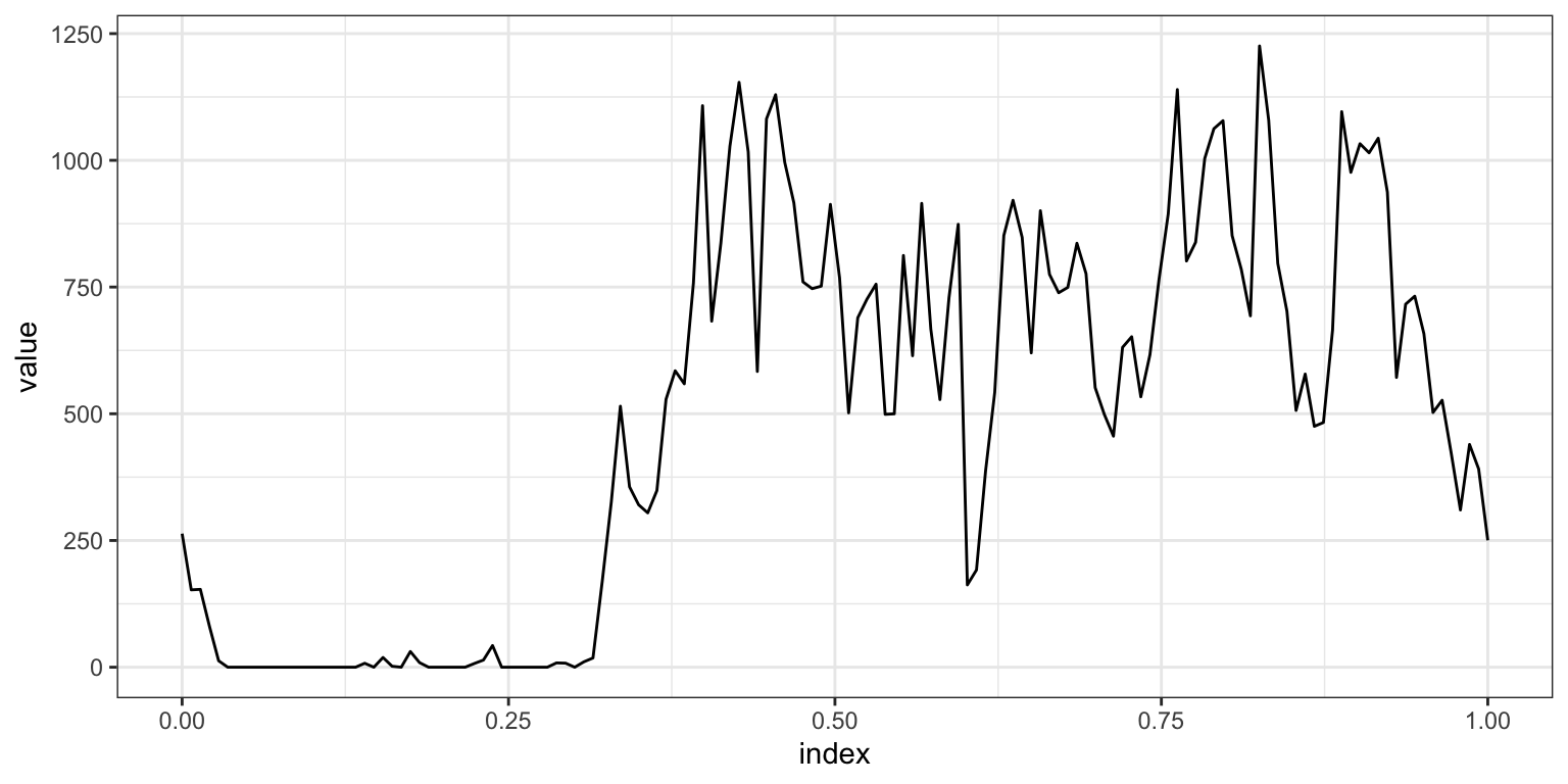

Next, we plot all subjects. The previous plot is a single noodle in this plot of spaghetti.

as_refundObj(accel) %>% 
    ggplot(aes(x = index, y = value, group = id)) + geom_path(alpha = .1)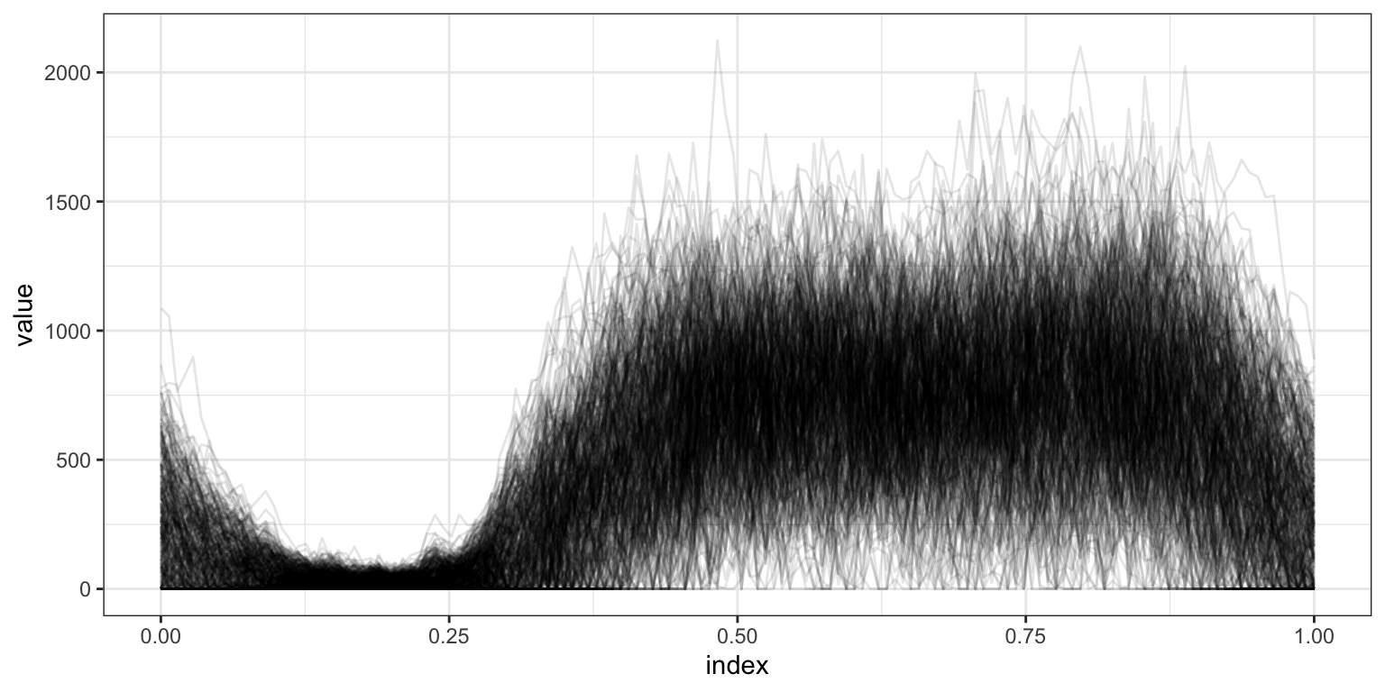

Now we compute the mean at each time point separately, and add this to our spaghetti.

pw_mean = as_refundObj(accel) %>%
    group_by(index) %>%
    summarize(pw_mean = mean(value))

as_refundObj(accel) %>% 
    ggplot(aes(x = index, y = value, group = id)) + geom_path(alpha = .1) +
    geom_path(data = pw_mean, aes(y = pw_mean, group = NULL), color = "red", size = 1)
## Warning: Using `size` aesthetic for lines was deprecated in
## ggplot2 3.4.0.
## ℹ Please use `linewidth` instead.
## This warning is displayed once every 8 hours.
## Call `lifecycle::last_lifecycle_warnings()` to see where
## this warning was generated.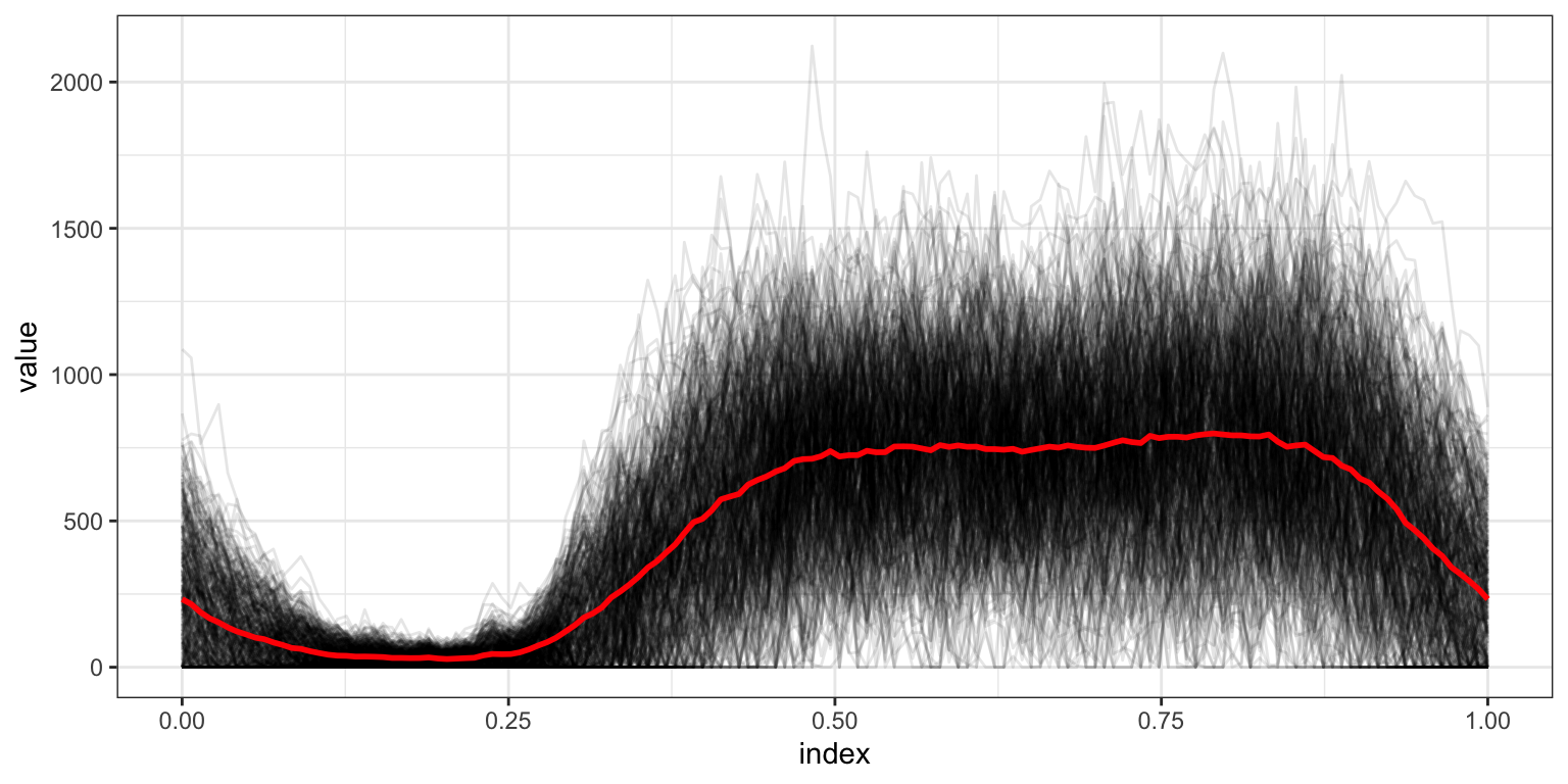

The pointwise mean is a bit jagged; now we use a smooth mean estimate.

as_refundObj(accel) %>% 
    ggplot(aes(x = index, y = value, group = id)) + geom_path(alpha = .1) +
    geom_smooth(aes(group = NULL), color = "red", size = 1) 
## `geom_smooth()` using method = 'gam' and formula = 'y ~
## s(x, bs = "cs")'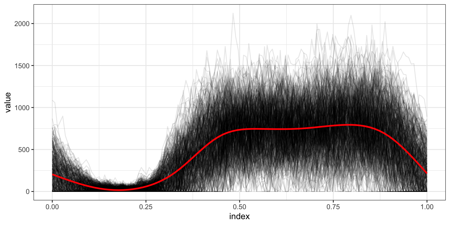

Rainbow plots color each noodle according to some covariate value. We illustrate this using BMI Z-score.

as_refundObj(accel) %>% 
    left_join(dplyr::select(covariate_data, id, BMIZ)) %>%
    ggplot(aes(x = index, y = value, group = id, color = BMIZ)) + geom_path(alpha = .5) + 
  scale_colour_gradientn(colours = c("red","yellow","green","lightblue","darkblue"),
                         values = c(1.0, 0.6, 0.55, 0.45, 0.4, 0))
## Joining with `by = join_by(id)`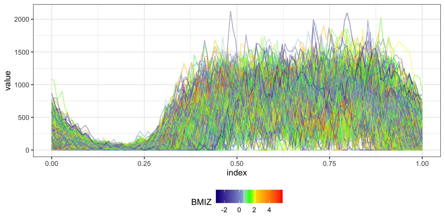

Lastly, we show the covariance surface to get an idea of the overall variance and the correlation across times.

library(plotly)
## 
## Attaching package: 'plotly'
## The following object is masked from 'package:grpreg':
## 
##     select
## The following object is masked from 'package:ggplot2':
## 
##     last_plot
## The following object is masked from 'package:stats':
## 
##     filter
## The following object is masked from 'package:graphics':
## 
##     layout

covariance = cov(accel)
plot_ly(z = ~covariance) %>% add_surface()