tidyfun
This page hosts a presentation / quick intro to tidyfun –
enjoy!
Example usage
The code in this page is drawn from tidyfun
vignettes, and is intended as a quick introduction; for more details,
please read the complete documentation!
If you haven’t installed tidyfun the code below will do
so.
devtools::install_github("tidyfun/tidyfun")Next I’ll load the package, as well as the
tidyverse.
library(tidyfun)
## Loading required package: tf
##
## Attaching package: 'tf'
## The following objects are masked from 'package:stats':
##
##     sd, var
## Registered S3 method overwritten by 'GGally':
##   method from
##   +.gg   ggplot2
library(refundr)
##
## Attaching package: 'refundr'
## The following objects are masked from 'package:tidyfun':
##
##     chf_df, dti_df
library(tidyverse)
Illustrative datasets
The datasets used in this vignette are the
tidyfun::chf_df and tidyfun::dti_df dataset.
The first contains minute-by-minute observations of log activity counts
(stored as a tfd vector called activity) over
seven days for each of 47 subjects with congestive heart failure. In
addition to id and activity, we observe
several covariates.
data(chf_df)A quick plot of these data is below.
chf_df %>%
  ggplot(aes(y = activity)) +
    geom_spaghetti(alpha = .05)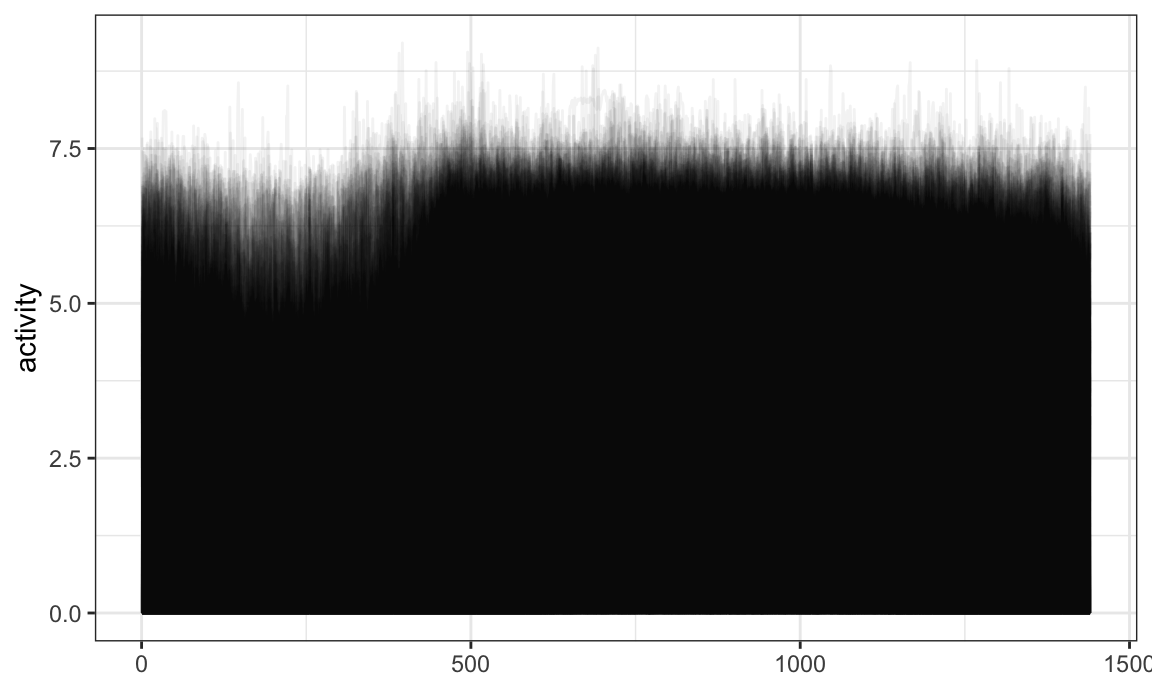
The tidyfun::dti_df contains fractional anisotropy (FA)
tract profiles for the corpus callosum (cca) and the right corticospinal
tract (rcst), along with several covariates.
data(dti_df)A quick plot of the cca tract profiles is below.
dti_df %>%
  ggplot(aes(y = cca)) +
    geom_spaghetti(alpha = .05)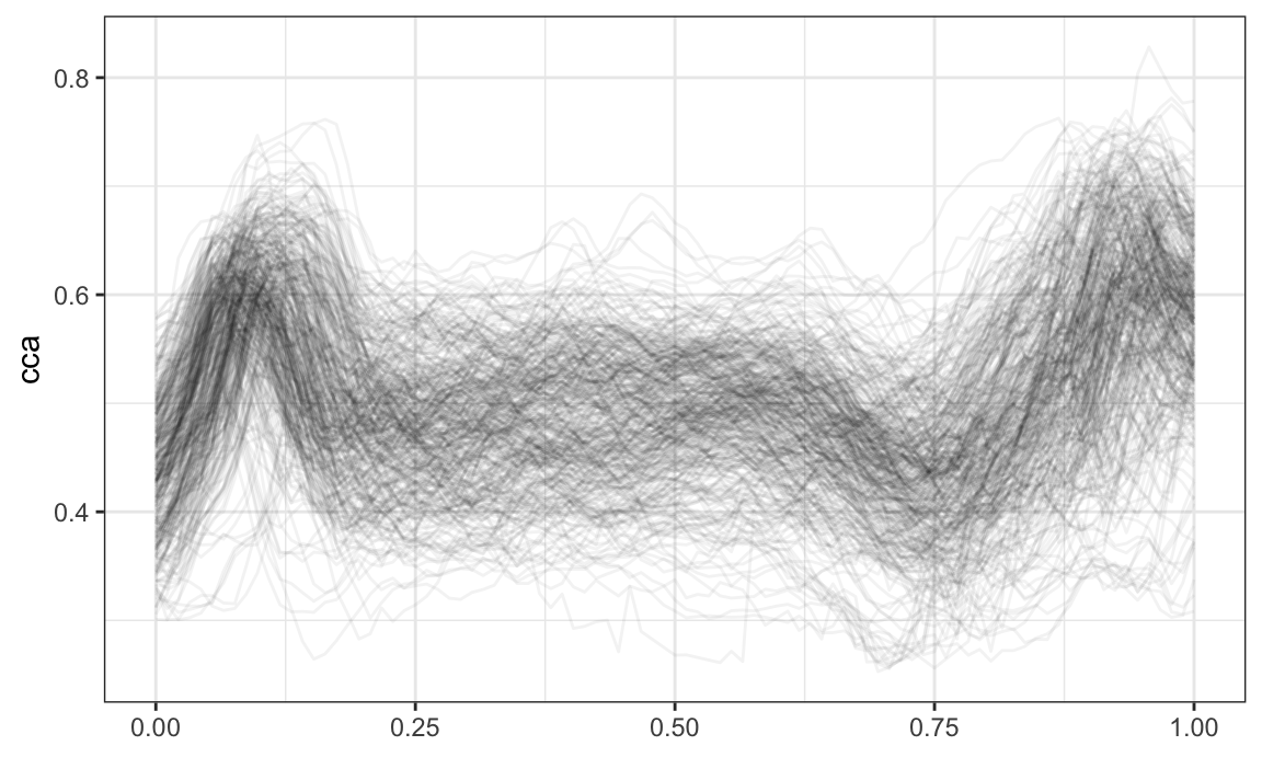
tf vectors
tf is a new data type for (vectors of)
functional data. It contains subclasses for “raw” functional data
(tfd) that can be dense / sparse and regular / irregular,
and for “basis representation” functional data (tfb).
Internally, there are attributes that define function-like
behavior, including evaluation for new arguments, resolution, and the
functional domain.
First I’ll pull a tf vector from the
tidyfun::dti_df dataset. The resulting vector contain
fractional anisotropy tract profiles for the corpus callosum
(cca). When printed, tf vectors show the first
few arg and value pairs for each subject.
data("dti_df")

cca_five = dti_df$cca[1:5]
cca_five
## irregular tfd[5] on (0,1) based on 93 to 93 (mean: 93) evaluations each
## interpolation by tf_approx_linear
## 1001_1: (0.000,0.49);(0.011,0.52);(0.022,0.54); ...
## 1002_1: (0.000,0.47);(0.011,0.49);(0.022,0.50); ...
## 1003_1: (0.000,0.50);(0.011,0.51);(0.022,0.54); ...
## 1004_1: (0.000,0.40);(0.011,0.42);(0.022,0.44); ...
## 1005_1: (0.000,0.40);(0.011,0.41);(0.022,0.40); ...
Converting “raw” to “basis” representation is possible, and introduces some smoothing by default.
cca_five_b =
  cca_five %>%
  tfb()
## Percentage of input data variability preserved in basis representation
## (per functional observation, approximate):
##    Min. 1st Qu.  Median    Mean 3rd Qu.    Max.
##   95.60   96.40   96.90   97.12   98.00   98.70
Operations on tf vectors
The following is a brief overview of the kinds of operations
available for tf vectors.
You can perform basic arithmetic and logical comparisons:
cca_five[1] + cca_five[1] == 2 * cca_five[1]
## 1001_1
##   TRUE
log(exp(cca_five[2])) == cca_five[2]
## 1002_1
##   TRUE
cca_five - (2:-2) != cca_five
## 1001_1 1002_1 1003_1 1004_1 1005_1
##   TRUE   TRUE  FALSE   TRUE   TRUE
You can summarize using mean, sd, and other
functions:
c(mean = mean(cca_five), sd = sd(cca_five))
## irregular tfd[2] on (0,1) based on 93 to 93 (mean: 93) evaluations each
## interpolation by tf_approx_linear
## mean: (0.000, 0.45);(0.011, 0.47);(0.022, 0.48); ...
## sd: (0.000,0.049);(0.011,0.052);(0.022,0.062); ...
You can determine whether a function satisfies a logical condition anywhere:
cca_five %>%
  tf_anywhere(value > .65)
## 1001_1 1002_1 1003_1 1004_1 1005_1
##   TRUE  FALSE   TRUE  FALSE  FALSE
And you can zoom in on regions of interest:
cca_five_zoom =
  cca_five %>%
  tf_zoom(.5, 1)

plot(cca_five_zoom)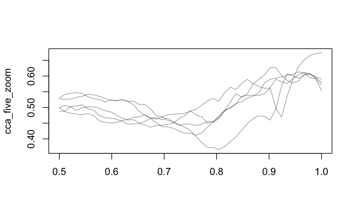
tf vectors in dataframes
The main goal of tidyfun is to ease exploratory analysis
by putting functional data in data frames. Since tf vectors
are treated the same way as vectors of class numeric or
factor, they can enter dataframes the same way.
The DTI data, for example, include scalar covariates and two functional variables:
dti_df
## # A tibble: 382 × 6
##       id visit sex    case                                                  cca
##    <dbl> <int> <fct>  <fct>                                          <tfd_irrg>
##  1  1001     1 female control  [1]: (0.000,0.49);(0.011,0.52);(0.022,0.54); ...
##  2  1002     1 female control  [2]: (0.000,0.47);(0.011,0.49);(0.022,0.50); ...
##  3  1003     1 male   control  [3]: (0.000,0.50);(0.011,0.51);(0.022,0.54); ...
##  4  1004     1 male   control  [4]: (0.000,0.40);(0.011,0.42);(0.022,0.44); ...
##  5  1005     1 male   control  [5]: (0.000,0.40);(0.011,0.41);(0.022,0.40); ...
##  6  1006     1 male   control  [6]: (0.000,0.45);(0.011,0.45);(0.022,0.46); ...
##  7  1007     1 male   control  [7]: (0.000,0.55);(0.011,0.56);(0.022,0.56); ...
##  8  1008     1 male   control  [8]: (0.000,0.45);(0.011,0.48);(0.022,0.50); ...
##  9  1009     1 male   control  [9]: (0.000,0.50);(0.011,0.51);(0.022,0.52); ...
## 10  1010     1 male   control [10]: (0.000,0.46);(0.011,0.47);(0.022,0.48); ...
## # ℹ 372 more rows
## # ℹ 1 more variable: rcst <tfd_irrg>
And the CHF data is an example of a multilevel dataset with a functional observation:
chf_df
## # A tibble: 329 × 8
##       id gender   age   bmi event_week event_type day
##    <dbl> <chr>  <dbl> <dbl>      <dbl> <chr>      <ord>
##  1     1 Male      41    26         41 .          Mon
##  2     1 Male      41    26         41 .          Tue
##  3     1 Male      41    26         41 .          Wed
##  4     1 Male      41    26         41 .          Thu
##  5     1 Male      41    26         41 .          Fri
##  6     1 Male      41    26         41 .          Sat
##  7     1 Male      41    26         41 .          Sun
##  8     3 Female    81    21         32 .          Mon
##  9     3 Female    81    21         32 .          Tue
## 10     3 Female    81    21         32 .          Wed
## # ℹ 319 more rows
## # ℹ 1 more variable: activity <tfd_reg>
Now our functional data are tidy! That is, we have data rectangles, and each functional observation exists in a single “cell”.
Data wrangling
Dataframes using tidyfun to store functional
observations can be manipulated using tools from dplyr,
including select and filter:
chf_df %>%
  select(id, day, activity) %>%
  filter(day == "Mon") %>%
  ggplot(aes(y = activity)) +
  geom_spaghetti(alpha = .05)
Operations using group_by and summarize are
allowed:
chf_df %>%
  group_by(day) %>%
  summarize(mean_act = mean(activity)) %>%
  ggplot(aes(y = mean_act, color = day)) +
  geom_spaghetti()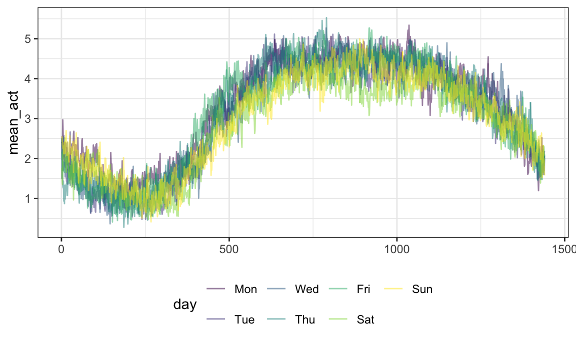
One can mutate functional observations – here we
exponentiate the log activity counts to obtain original recordings:
chf_df %>%
  mutate(exp_act = exp(activity)) %>%
  ggplot(aes(y = exp_act)) +
  geom_spaghetti(alpha = .05)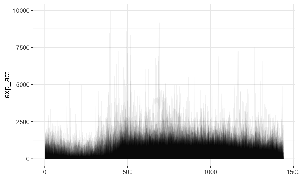
Some dplyr functions are most useful in conjunction with
new functions in tidyfun. For example, one might use
filter with tf_anywhere to filter based on the
values of observed functions:
chf_df %>%
  filter(tf_anywhere(activity, value > 9)) %>%
  ggplot(aes(y = activity)) +
  geom_spaghetti()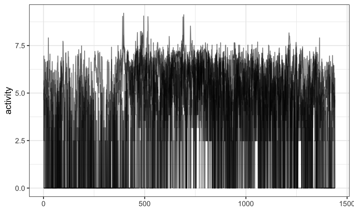
One can add smoothed versions of existing observations using
mutate and tf_smooth:
chf_df %>%
  filter(id == 1) %>%
  mutate(smooth_act = tf_smooth(activity)) %>%
  ggplot(aes(y = smooth_act)) +
  geom_spaghetti()
## using f = 0.15 as smoother span for lowess
## New names:
## • `.` -> `....1`
## • `.` -> `....2`
## • `.` -> `....3`
## • `.` -> `....4`
## • `.` -> `....5`
## • `.` -> `....6`
## • `.` -> `....7`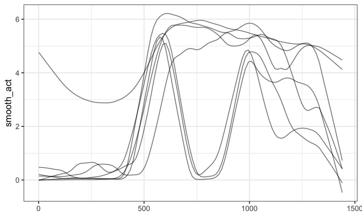
One can also extract observations over a subset of the full domain
using mutate and tf_zoom:
chf_df %>%
  filter(id == 1) %>%
  mutate(daytime_act = tf_zoom(activity, 360, 1200)) %>%
  ggplot(aes(y = daytime_act)) +
  geom_spaghetti()
## New names:
## • `.` -> `....1`
## • `.` -> `....2`
## • `.` -> `....3`
## • `.` -> `....4`
## • `.` -> `....5`
## • `.` -> `....6`
## • `.` -> `....7`
In general, EDA for functional data using tidyverse
tools is now possible, and is often most powerful when paired with new
functions in tidyfun.
Visualization
We’ve seen both plot and geom_spaghetti to
aid in understanding some content to this point – base R for
tf vectors, ggplot for tidy data. You can use
more advanced options and combine with data wrangling steps.
You can use facetting:
chf_df %>%
  filter(day %in% c("Mon", "Sun")) %>%
  ggplot(aes(y = activity, color = gender)) +
  geom_spaghetti(alpha = .1) +
  facet_grid(gender ~ day)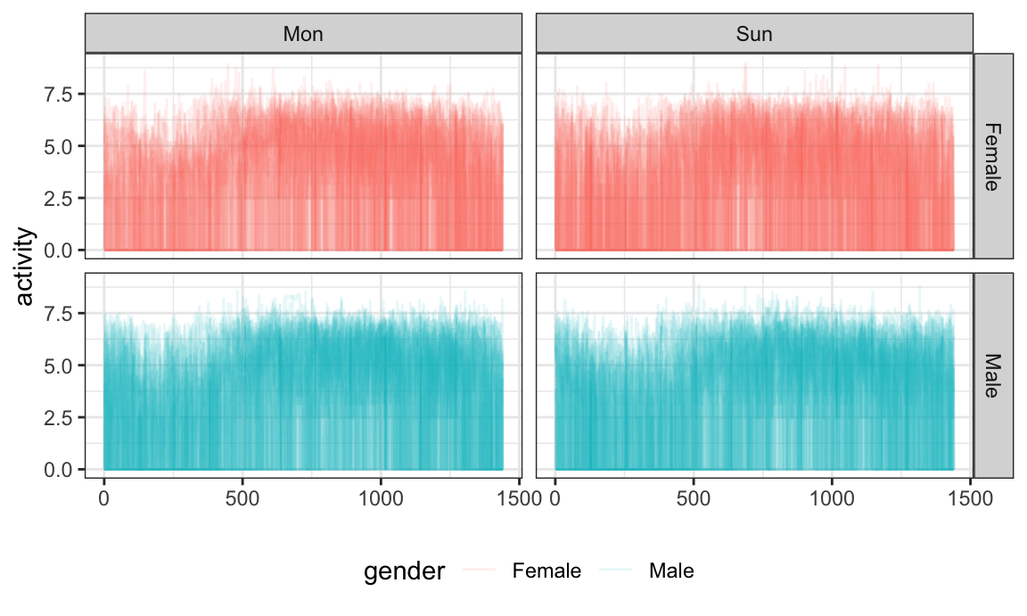
Together with data manipulation tools, the integration with
ggplot can produce useful exploratory analyses. Note that
this plot also introduces geom_meatballs():
chf_df %>%
  group_by(gender, day) %>%
  summarize(mean_act = mean(activity)) %>%
  mutate(smooth_mean = tfb(mean_act)) %>%
  filter(day %in% c("Mon", "Sun")) %>%
  ggplot(aes(y = smooth_mean, color = gender)) +
  geom_spaghetti(size = 1.25, alpha = 1) +
  geom_meatballs(aes(y = mean_act), alpha = .1) +
  facet_grid(~ day)
## `summarise()` has grouped output by 'gender'. You can
## override using the `.groups` argument.
## Percentage of input data variability preserved in basis
## representation (per functional observation, approximate):
## Min. 1st Qu.  Median Mean 3rd Qu.  Max.  88.70 91.35 92.00
## 91.56 92.25 93.00
## Percentage of input data variability preserved in basis
## representation (per functional observation, approximate):
## Min. 1st Qu.  Median Mean 3rd Qu.  Max.  89.00 91.80 93.00
## 92.14 93.05 93.30
## Warning in geom_spaghetti(size = 1.25, alpha = 1): Ignoring unknown parameters:
## `size`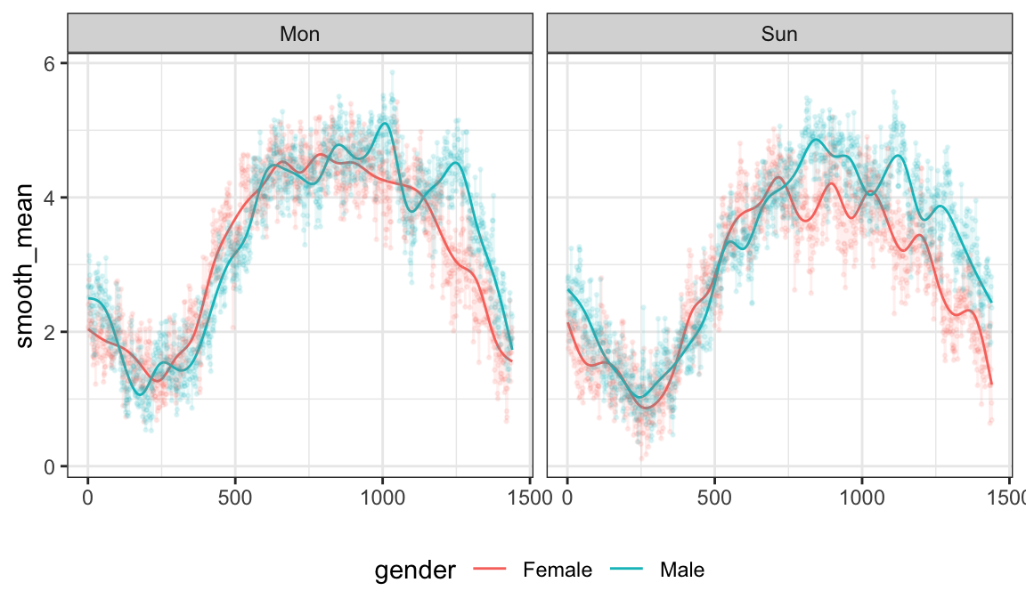
Lasagna plots are a variant on a heatmaps which show functional
observations in rows and use color to illustrate values taken at
different arguments. In tidyfun, lasagna plots are
implemented through gglasagna. A first example, using the
CHF data, is below.
chf_df %>%
  filter(day %in% c("Mon", "Sun")) %>%
  gglasagna(activity)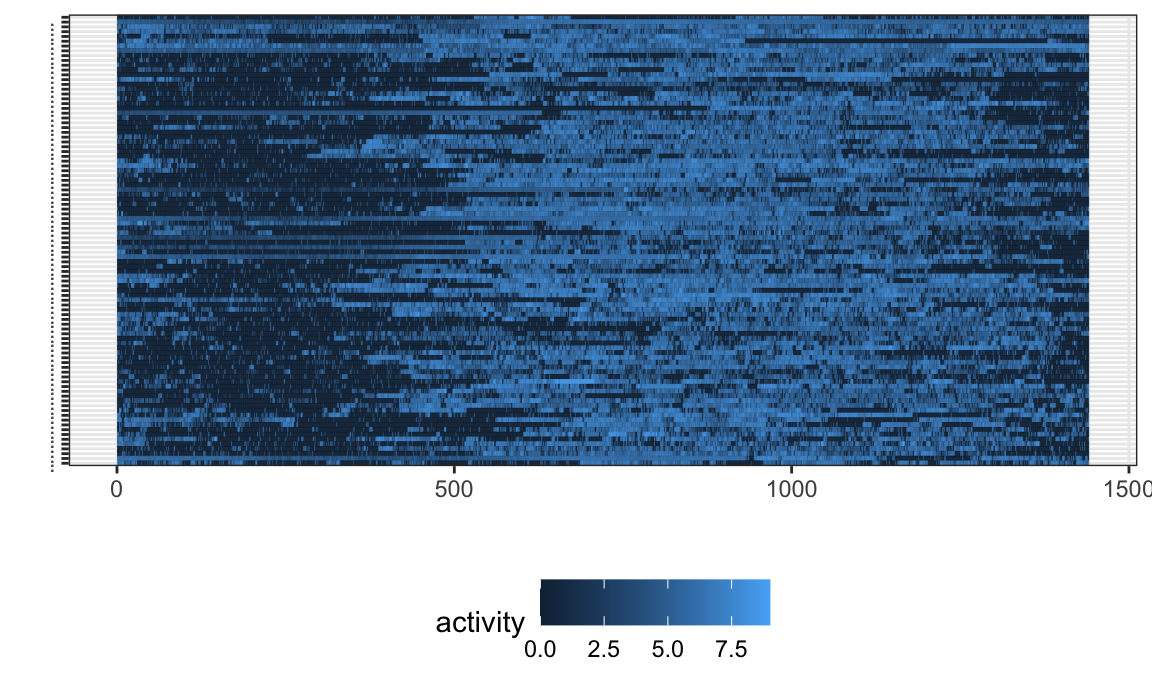
A somewhat more involved example, demonstrating the
order argument and taking advantage of facetting, is
next.
dti_df %>%
  gglasagna(
    tf = cca,
    order = tf_integrate(cca, definite = TRUE),
    arg = seq(0,1, l = 101)) +
  theme(axis.text.y = element_text(size = 6)) +
  facet_wrap(~ case, ncol = 2, scales = "free")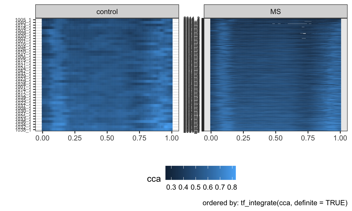
Conversion
The DTI data in the refund package has been
a popular example in functional data analysis. In the code below, we
create a data frame (or tibble) containing scalar
covariates, and then add columns for the cca and
rcst track profiles. This code was used to create the
tidyfun::dti_df dataset included in the package.
dti_df = tibble(
  id = refund::DTI$ID,
  sex = refund::DTI$sex,
  case = factor(ifelse(refund::DTI$case, "MS", "control")))

dti_df$cca = tfd(refund::DTI$cca, arg = seq(0,1, l = 93))
dti_df$rcst = tfd(refund::DTI$rcst, arg = seq(0, 1, l = 55))
“Long” format data frames containing functional data include columns
containing a subject identifier, the functional argument, and the value
each subject’s function takes at each argument. There are also often
(but not always) non-functional covariates that are repeated within a
subject. For data in this form, we use tf_nest to produce a
data frame containing a single row for each subject.
An example is the pig weight data from the SemiPar
package, which is a nice example from longitudinal data analysis. This
includes columns for id.num, num.weeks, and
weight – which correspond to the subject, argument, and
value.
data("pig.weights", package = "SemiPar")

pig.weights = as_tibble(pig.weights)

pig.weights
## # A tibble: 432 × 3
##    id.num num.weeks weight
##     <int>     <int>  <dbl>
##  1      1         1   24
##  2      1         2   32
##  3      1         3   39
##  4      1         4   42.5
##  5      1         5   48
##  6      1         6   54.5
##  7      1         7   61
##  8      1         8   65
##  9      1         9   72
## 10      2         1   22.5
## # ℹ 422 more rows
We create pig_df by nesting weight within subject. The
result is a data frame containing a single row for each pig, and columns
for id.num and the weight function.
pig_df =
  pig.weights %>%
  tf_nest(weight, .id = id.num, .arg = num.weeks)

pig_df
## # A tibble: 48 × 2
##    id.num                          weight
##     <int>                       <tfd_reg>
##  1      1  [1]: (1,24);(2,32);(3,39); ...
##  2      2  [2]: (1,22);(2,30);(3,40); ...
##  3      3  [3]: (1,22);(2,28);(3,36); ...
##  4      4  [4]: (1,24);(2,32);(3,40); ...
##  5      5  [5]: (1,24);(2,32);(3,37); ...
##  6      6  [6]: (1,23);(2,30);(3,36); ...
##  7      7  [7]: (1,22);(2,28);(3,36); ...
##  8      8  [8]: (1,24);(2,30);(3,38); ...
##  9      9  [9]: (1,20);(2,28);(3,33); ...
## 10     10 [10]: (1,26);(2,32);(3,40); ...
## # ℹ 38 more rows
Additional functions allow conversion from other data structures to
tf vectors, and also implement conversions back to these
data structures.
Next steps
tidyfun itself is a work in progress:
- There are several open issues / to dos / bug fixes
- We have some ideas for new features
- User feedback will help!
Integration with analysis is longer-term goal:
- Some
refundfunctions have been unofficially updated to work with dataframe /tfintpus - More robust / complete integration is needed