Scalar-on-Function Regression
This page contains a combination of traditional lecture materials (slides) and code demonstrating the relevant methods. The short course will proceed by working through both. We will use several recent packages in our examples; see the About page for information about the package versions.
library(tidyverse)
## ── Attaching packages ───────────────────────────────────────────────────────────────────────────────────────────────────────────────────────────────────────────────────────────────────────────────────────────────── tidyverse 1.2.1 ──
## ✔ ggplot2 3.2.1     ✔ purrr   0.3.3
## ✔ tibble  2.1.3     ✔ dplyr   0.8.3
## ✔ tidyr   1.0.0     ✔ stringr 1.4.0
## ✔ readr   1.3.1     ✔ forcats 0.4.0
## ── Conflicts ──────────────────────────────────────────────────────────────────────────────────────────────────────────────────────────────────────────────────────────────────────────────────────────────────── tidyverse_conflicts() ──
## ✖ dplyr::filter() masks stats::filter()
## ✖ dplyr::lag()    masks stats::lag()
library(grpreg)
##
## Attaching package: 'grpreg'
## The following object is masked from 'package:dplyr':
##
##     select
library(splines)
library(refund)
library(refund.shiny)
## This version of Shiny is designed to work with 'htmlwidgets' >= 1.5.
##     Please upgrade via install.packages('htmlwidgets').
In this section we’ll use the DTI dataset to motivate the scalar-on-function regression model and variable selection in this context. Our main outcome of interest is multiple sclerosis case status, and the possible predictors are tract profiles from several major white matter structures. Below we plot profiles for one tract colored by MS case status.
load("./DataCode/DTI.RDA")

as_refundObj(CCA_ani) %>%
    left_join(dplyr::select(outcome_data, id, case)) %>%
    ggplot(aes(x = index, y = value, group = id, color = case)) + geom_path(alpha = .5)
## Joining, by = "id"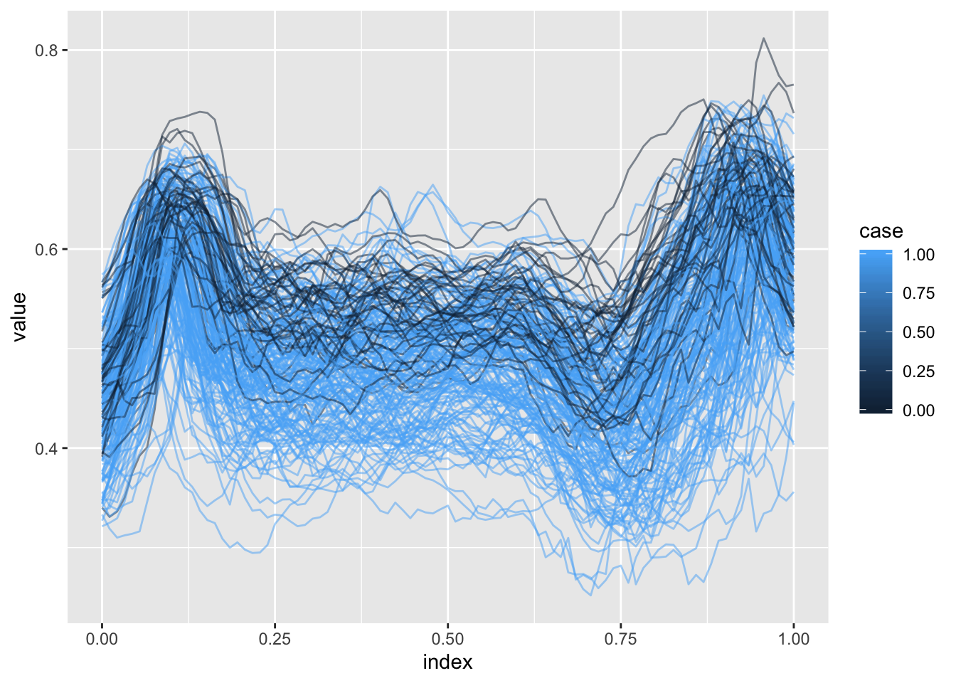
Methods for variable selection
Slides below review scalar-on-function regression and introduce the ideas for variable selection in this context.
Practical example
Some DTI profiles are incomplete; we can use FPCA to obtain estimates over a complete domain.
fpca_ex = fpca.sc(CSTL_ani)

bind_rows(as_refundObj(fpca_ex$Y) %>% mutate(type = "Observed"),
                    as_refundObj(fpca_ex$Yhat) %>% mutate(type = "Fitted")) %>%
    ggplot(aes(x = index, y = value, group = id)) + geom_path(alpha = .5) +
        facet_grid(~type)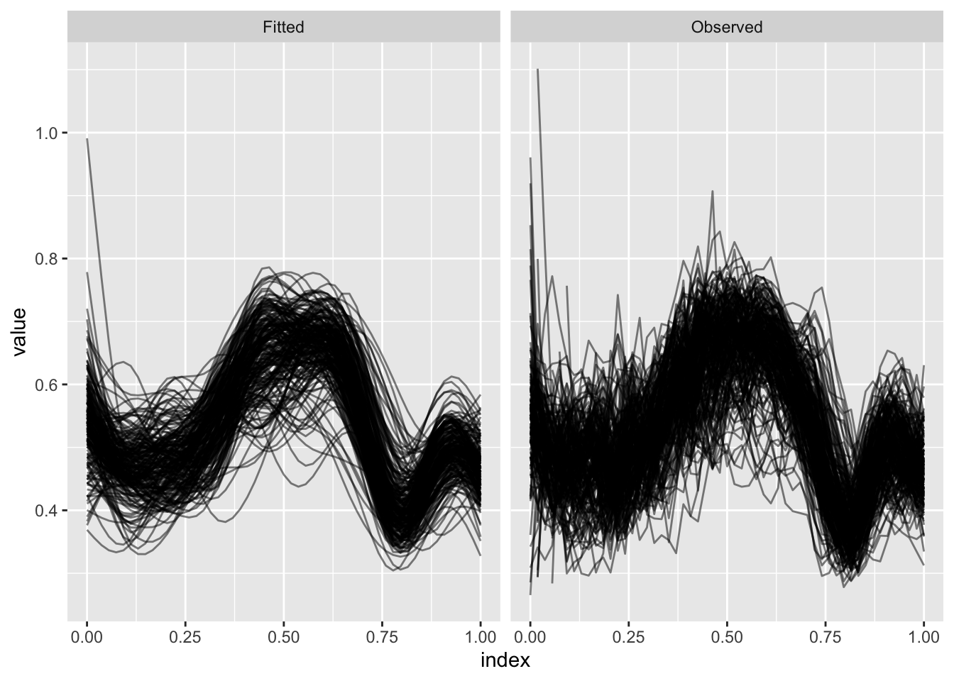
(Incidentally, the refund.shiny package has helpful tools for visualizing the results of an FPCA analysis. More information about the package can be found here.)
plot_shiny(fpca_ex)Several steps are needed to organize the functional predictors to fit the scalar-on-function regression with variable selection. In particular, for this dataset we use FPCA on each predictor; scale the resulting reconstructions; and combine with a spline basis. The code below implements these steps and produces a list containing the result for each predictor.
basis_create = function(data_matrix) {
    index = seq(0, 1, length = dim(data_matrix)[2])
    basis = splines::bs(index, df = 10, intercept = TRUE)
}

preprocess_fd_for_sofr = function(data_matrix, basis){

    int_weights = rep(1 / dim(data_matrix)[2], dim(data_matrix)[2])

    fitted_vals = fpca.sc(data_matrix, npc = 10)$Yhat
    scaled_fv = scale(fitted_vals)

    design_mat = scaled_fv %*% diag(int_weights) %*% basis
}

predictor_names = paste(rep(c("CSTR", "CSTL", "CCA", "OPRL", "OPRR"), each = 6),
                                    rep(c("ani", "l0", "lt", "md", "mtr", "t2"), 5),
                                    sep = "_")

predictors = map(predictor_names, get)
predictor_basis = map(predictors, basis_create)

processed_predictors = map2(predictors, predictor_basis, preprocess_fd_for_sofr)
Given the processed predictors, we construct the design matrix and fit the model using the group variable selection illustrated previously.
y = outcome_data$case
X = do.call(cbind, processed_predictors)
group = factor(rep(predictor_names, each = 10), levels = predictor_names)

sofr_fit = grpreg(X = X, y = y, group = group, family = "binomial", penalty = "grLasso")
The panels below show the results of the preceding model fit for two values of the tuning parameter. For each, estimated spline coefficients are combined with the spline basis to produce the coefficient function.
single_coef_construct = function(coefs, basis, name) {
    coef_data_frame = data.frame(
      value = basis %*% coefs,
      index = seq(0, 1, length = dim(basis)[1]),
      id = name,
      stringsAsFactors = FALSE
    )
}

coef_construct = function(lambda_index) {
    arg_list = list(split(sofr_fit$beta[-1, lambda_index], group),
                                    predictor_basis,
                                    predictor_names)
    pmap(arg_list, single_coef_construct) %>%
    bind_rows %>%
    mutate(lambda = round(sofr_fit$lambda[lambda_index], 3))
}

bind_rows(coef_construct(30), coef_construct(90)) %>%
    ggplot(aes(x = index, y = value, group = id)) + geom_path() +
    facet_grid(~lambda)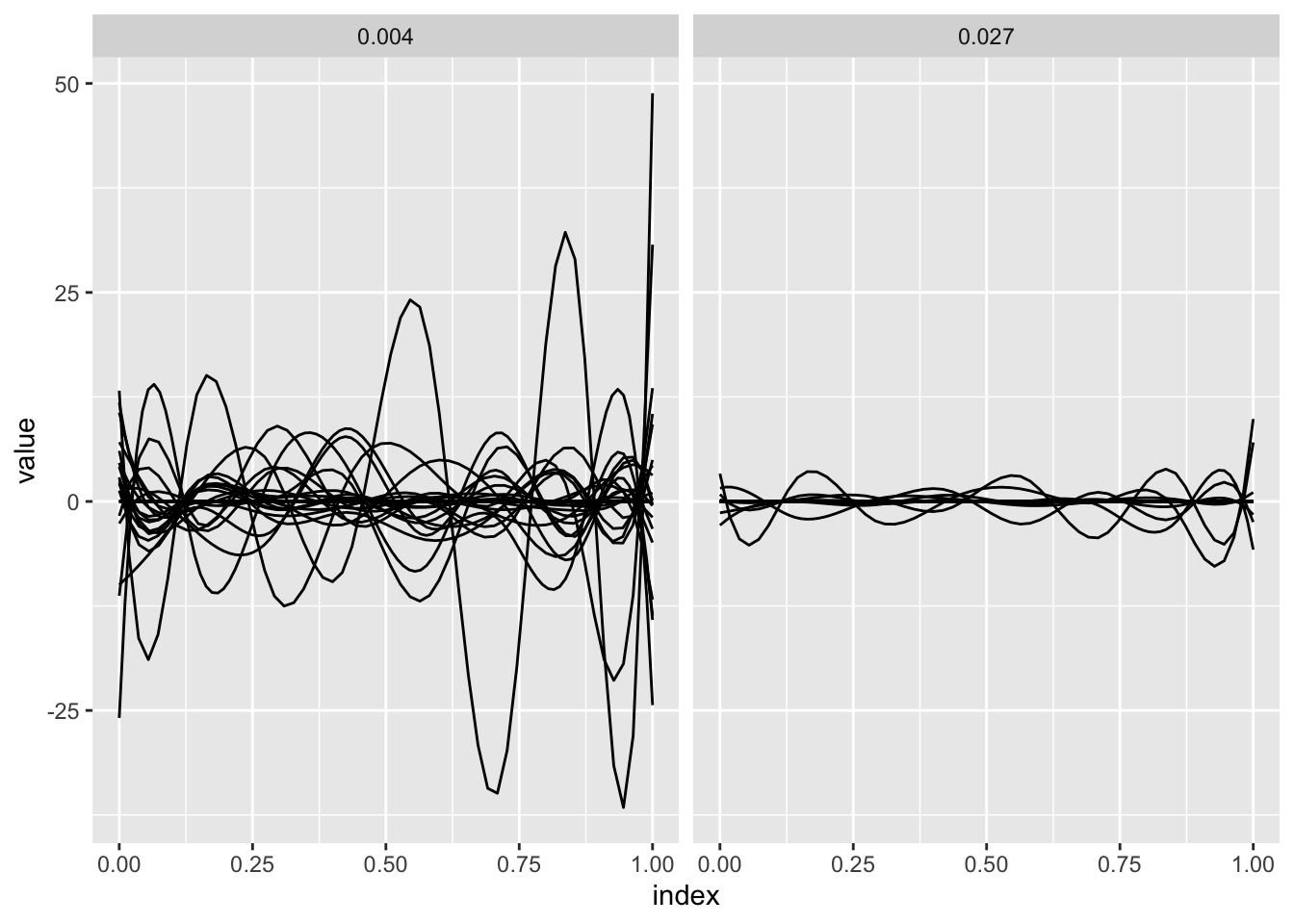
Try it yourself!
Another example for variable selection in the scalar-on-function regression setting is the Sugar dataset. In this example, predicting the ash content of a sugar sample based on emission spectra at several wavelengths (and on the derivatives of these spectra) is of interest.
Below we plot the spectra at a single wavelength colored by ash content.
load("./DataCode/Sugar.RDA")

as_refundObj(wave_230) %>%
    left_join(dplyr::select(outcome_data, id, ash)) %>%
    ggplot(aes(x = index, y = value, group = id, color = ash)) + geom_path(alpha = .5)
## Joining, by = "id"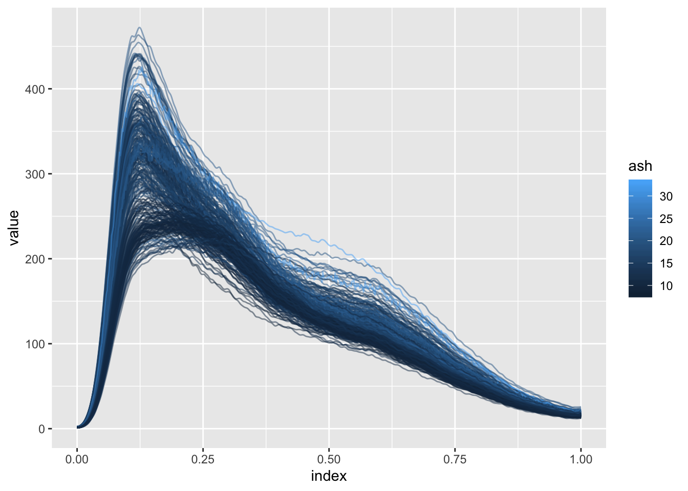
You’re encouraged to try the preceeding variable selection tools on these data, and to extend them in directions that interest you. You may also be interested in exploring the use of methods in Gertheiss et al (2013); code implementing these methods for the DTI and Sugar data is available here.